Adaptive short term forecasting

Truth be told, I’m more a business user then mathematician or programmer. Thus the proposed algorythm is more “I see like this” practice then mathematically and statistically stuffed theory. Hovewer this algorytm can be a usefull example of a mix of popular machine learning techniques into adaptive auto-regression forecasting model.

First glance on the data

Input data for forecasting is daily delinquency bucket volumes since 2013 - all in all 14 time series which are correlated with the neighbour with some lag. Usually this lag is around 30 days, but not always.

On the table below you can see the example of one of the time series. Rows are days, columns are months. White squares are weekends/holidays or were excluded as outliers (outliers are covered in the next part). You can also see that the time series have dual seasonality (weekly and monthly) and trend.

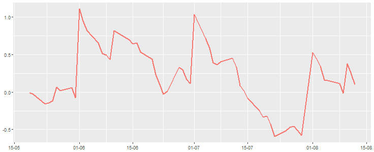
Each time series has its unique trend, seasonality and variance. As you can see on the chart below, the variance can be really high. Below is the example of one of the normalized time series

The task is to develop an algorithm which will predict Y for the next month for each time series with Mean Absolute Percentage Error (MAPE) < 3%.

Forecasting algorithm

Some reseaches assume that there are around 100 forecasting model types. Probably this number is overestimated, however we must admit that the number of model types is high and below is presented only main one:

• Auto-regression models and moving average (ARMA, ARIMA, GARCH, etc.)
• SSA/Gusenitca
• Neural networks (RNN)
• Adaptive short term forecasting:
  • Exponential smoothing;
  • Seasonal and trend decomposition;
  • Adaptive auto-regression;
• Adaptive model selection & composition.

First my thought was not to overcomplicate the task and to decompose time series by trend and seasonality. There is a great forecast package, developed by Rob Hyndman, which can do it for you. TBATS is the one algorithm from this package which can decompose dual seasonality. But the problem is that you need to somehow approach missing values without loosing accuracy and include lagged correlated time series as regressors. That’s why I transformed the task to regression task, which is well known and was solved million of times.

Following algorithms were chosen as challengers:

0.Dimension reduction (Principal Component Analysis - PCA).

1.Ensembles (Random Forest, Gradient Boosted Models - GBM and XGBoost);

2.Regressions (Linear, Stepwise, Ridge and Lasso);

3.Distance based (k-Nearest Neighbor - kNN);

Whole forecasting algorithm is presented below:

The algorithm starts with data preparation, then feature engineering and modeling. The last part is forecasting itself. In order to build a forecast, each new period of forecasting must have previous forecasting results as input, that’s why additional inner loop by number of periods ahead was added to forecasting algorithm.

Data preparation and new features

First of all, you need to normalize data and remove outliers.

Normalization not only helps to increase the speed of some algorithms (such as gradient descent) but also is essential for distance based algorithms. For example for this research, normalization (I used the one based on standard deviation) made possible for penalized regression to outperform regular regression.

Outliers makes noise in data and depending on the context, they either deserve special attention or should be completely ignored. Some models are more sensitive to outliers than others. I’ve removed outliers from train samples based on both 3-sigma rule and business logic and this helped to increase accuracy on test samples by 3% in average.

Observation period. For regular machine learning task there is a plato in learning capabilities if we increase the amount of input data (I must note that this is not the case for deep learning, however in this task I’ve not used it). Thus minimal observation period was set as 2 years of daily data based on validation results.

Observation period can be optimized via validation

From 90 to 120 new features were created for each time series. Most of them are lagged values of correlated buckets, you can see sample code of the function below. Calendar features are the variables which I created from calendar (number of a day, number of a working day, number of a month, number of days since last working day, etc.). You also need to define how you want to treat you calendar features. The best way is to keep them as continuous, but sometimes it make sense to cast them into factors, this can help to model nonlinear relationships in linear models. If you cast variables to factors you need to keep in mind that for some models you need to make on-hot-encoding and convert you X data to numeric matrix (e.g. penalized regression, gradient boosting).

X_lagged_create<-function(bucket_name,actual_date,Y){
  X_lagged<-NULL
  for (i in 1:3){ 
    bucket_name_i<-as.character(buckets[buckets$this_bk==bucket_name,i])
    if(is.na(bucket_name_i)==F){
      lag_values<-data.frame(actual_date=Y[,1],value=Y[,bucket_name_i])
      lag_values<-merge(lag_dates,lag_values,by.x="lag_date",by.y="actual_date")
      lag_values$var_name<-paste0(colnames(buckets)[i],"_",lag_values$variable)
      X_lagged<-rbind(X_lagged,lag_values)
    }
  }
  X_lagged<-dcast(X_lagged,actual_date~var_name,mean)
  X_lagged<-X_lagged[match(actual_date,X_lagged[,1]),]
  X_lagged[,1]<-NULL
  return(X_lagged)
}

Do not hesitate to use hundreds or even thousand of features. If you are afraid that your algorithm will slow down - use data.table package. On the example above you can see dcast function from data.table package instead and cast from reshape. This reduced time spent on this operation 4 times - from 4 seconds to 1 second.

Modeling

Accuracy measure

First of all, before modeling time series,you need to choose accuracy measure which will define best model. One of the most popular measure is Mean Absolute Percentage Error (MAPE). MAPE is often preferred because apparently managers understand percentages better than squared errors. However it falls then you need to compare time series which are close to zero - it just blows up due denominator. This is our case as we scaled time series around 0. Thus Mean Squared Error (MSE) was chosen as a measure of accuracy:

mse<-function(y_pred,y_test){
  return(mean((y_pred-y_test)**2))
}

Work on your coding skills. Your code needs to be readable, maintainable, testable and elegant. Copy-pasting is prohibited, functions and clear naming are encouraged. Save results of every experiment even if it fails. This lecture is a good place to start

Weights

The hypothesis behind weights is that some observations are more reliable then the others and can reveal data structure better. And this make sense, especially for forecasting, when trends can change each 2-3 seasons. The value of weights can be assigned judgmentally to each observation. I used following linear formula, which basically says to treat more recent observations as twice more important then observations 2 years ago:

weights_lm<-(1:nrow(X_train))*(1/nrow(X_train))+1

After you calculated weights you can either assign them via sampling or put them inside algorithm if it supports weighing. I’ve chosen second option and error rate decreased by roughly 4%.

Dimension reduction

The transformation of the data, by centering, rotating and scaling informed by PCA can improve the convergence time and the quality of results. In theory the PCA makes no difference, but in practice it improves rate of training, simplifies the model structure to represent the data, and results in systems that better characterize the “intermediate structure” of the data instead of having to account for multiple scales - it is more accurate. Below is the sample code of PCA:

X_train_pca <- prcomp(get_matrix(X_train))
summary(X_train_pca)
X_test_pca<-predict(X_train_pca,get_matrix(X_test))

Some take aways from modeling:

1. Regular linear model:

fit_lm <- lm(y_train~.,X_train,weights = weights_lm)
summary(fit_lm)
y_train_pred<-predict(fit_lm,X_train)
y_test_pred<-predict(fit_lm,X_test)

The model showed pretty good results, it is prone to overfitting. However do not guarantee you best results without proper feature selection while multicollinearity can spoil all the fun from modeling. This is where stepwise and penalized regressions step into.

2. Stepwise regression

Stepwise regression demonstrated results which were on average 1-2% better then regular linear model. But the problem (and this is really big problem) is that it really time consuming! For 14 time series and 90-120 variables for each time series it requires total 22 minutes (!) on Intel Core i5 4 GB RAM to solve the model. Below is the example of backward stepwise regression:

fit_lm <- lm(y_train~.,X_train,weights = weights_lm)
fit_lm_clean<-step(fit_lm,direction="backward",test="F",trace=F,weights = weights_lm)
y_train_pred<-predict(fit_lm_clean,X_train)
y_test_pred<-predict(fit_lm_clean,X_test) 

3. Penalized regression

Penalization decreased error by 11% comparing with regular linear model. The algorithm is extremely fast, for same task on same PC it requires just 3.3 seconds (not even minutes). However you need to keep in mind that it works perfectly on normalized data and requires lambda (regularization parameter) and alpha (which defines if it’s ridge or lasso penalty) optimization:

library(glmnet)	 
fit_glmnet <- glmnet(get_matrix(X_train), y_train,weights = weights_lm)
y_train_pred<-predict(fit_glmnet,get_matrix(X_train),s=0.005)
y_test_pred<-predict(fit_glmnet,get_matrix(X_test),s=0.005)

4. Trees

I like building tree models, it can be simple c4.5, CART, more advanced Random Forest or even Gradient Boosted Models (GBM) and XGBoost. And boosted trees are my favorite models, which I try to put in every task. However you need to be very mindful and accurate while building tree. Tree algorithms do not provide any statistical significance measures and can be easily overfitted. Sometimes even if you do shallow trees with 2-4 layers, define minimum number of observations in nodes, optimize learning rate and number of variables via cross validation, the trees just do not work. Below is the example of XGBoost code with cross validation of deepness:

library(xgboost)
xgbMatrix <- xgb.DMatrix(data=X_train, 
                           label = y_train, 
                           weight = weights_lm)
cv_xgboost <- xgb.cv(data=xgbMatrix,
                         nfold = 5, maximize = FALSE,  early.stop.round = 8,
                          nrounds = 1200, objective ="reg:linear", max.depth = 4,
                          eta = 0.1, min_child_weight = 20,colsample_bytree = 0.1)
fit_xgboost <- xgboost(data=xgbMatrix,
                       nrounds = nrow(cv_xgboost), objective ="reg:linear", max.depth = 4,
                       eta = 0.1, min_child_weight = 20,colsample_bytree = 0.1)
importance_matrix <- xgb.importance(feature_names =colnames(X_train), model = fit_xgboost)
xgb.plot.importance(head(importance_matrix,10))
y_train_pred<-predict(fit_xgboost,X_train)
y_test_pred<-predict(fit_xgboost,X_test)

Take care of proper validation. Precise model can be overfitted even If it was developed and tested on different populations (that’s why I do not like Kaggle much:)). You need to have at least 5 out-of-time (OOT) samples from different periods. Of course, for each iteration you need to take OOT sample as of most recent period and develop a model based on previous period.

5. kNN

k-Nearest Neighbors is simple but relible algorithm. Unfortunatelly it didn’t show any positive results during this research. However it can be used as input for other algorithms. Or we can calculate weights based on nearest months to the forecasting period usung kNN.

library(FNN)
knn_perf<-NULL
for (k_i in 1:40) {
  y_test_pred<-knn.reg(X_train,X_test,y_train,k=k_i)[[4]]
  knn_perf_i<-data.table(k=k_i,mse=mse(y_test_pred,y_test))
  knn_perf<-rbind(knn_perf,knn_perf_i)
}
k_final<-which.min( knn_perf$mse ) 
y_train_pred<-knn.reg(X_train,X_train,y_train,k=k_final)[[4]]
y_test_pred<-knn.reg(X_train,X_test,y_train,k=k_final)[[4]]

Final results & summary

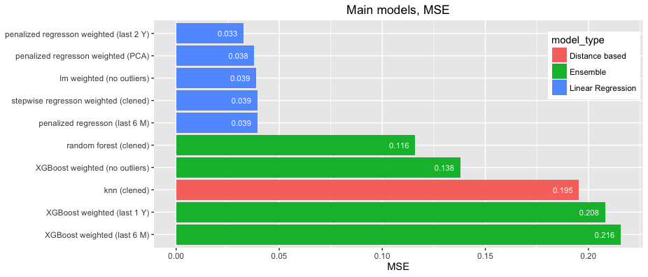
Totally was created around 2k models, which wont’t fit to any chart unless you clusterize them:), so only main algorithms are presented below:

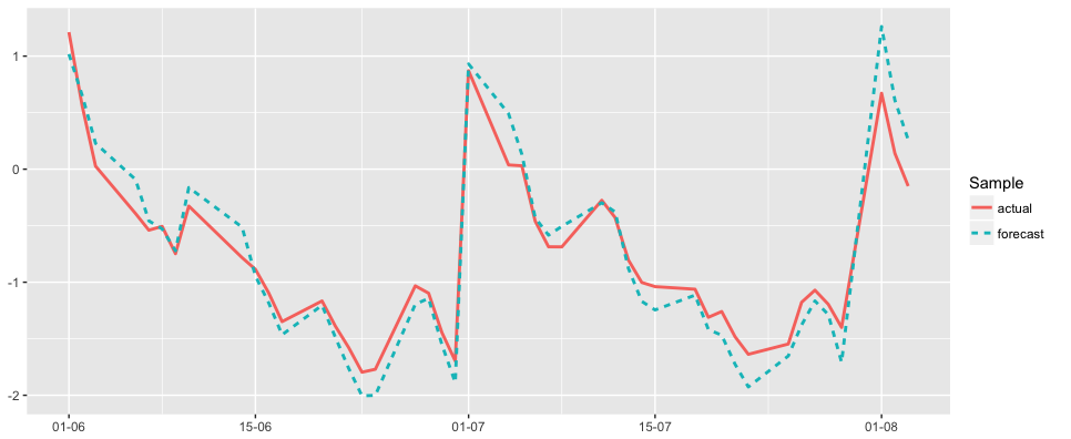
As a result of testing, weighted penalized regression was chosen as base algorithm with α=0 (ridge regression) and λ=0.005. Observation period was set as 2 years.

The proposed algorithm allows to build time series forecasting of multiple interdependent time series. It automatically reveals any kind of seasonality, deals with missing values/outliers and removes overfitting/multicollinearity via penalization. It’s scalable for new features (both lagged and calendar), period of forecasting and number of interdependent time series.

What can be tested further?

• weights assigned based on nearest month via kNN algorythm
• RNN/LSTM
• seasonality and trend decomposition via TBATS package